Polynomial regression using statsmodel ·

I’ve been using sci-kit learn for a while, but it is heavily abstracted for getting quick results for machine learning. Particularly, sklearn doesnt provide statistical inference of model parameters such as ‘standard errors’. Statsmodel package is rich with descriptive statistics and provides number of models.

Let’s implement Polynomial Regression using statsmodel

Import basic packages

import numpy as np
import matplotlib.pyplot as plt
import pandas as pd

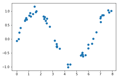
Create artificial data

rng = np.random.RandomState(1)
x = 8 * rng.rand(50)
y = np.sin(x) + 0.1 * rng.randn(50)

#Create single dimension
x= x[:,np.newaxis]
y= y[:,np.newaxis]

inds = x.ravel().argsort()  # Sort x values and get index    
x = x.ravel()[inds].reshape(-1,1)
y = y[inds] #Sort y according to x sorted index

print(x.shape)
print(y.shape)

#Plot
plt.scatter(x,y)

(50, 1)
(50, 1)

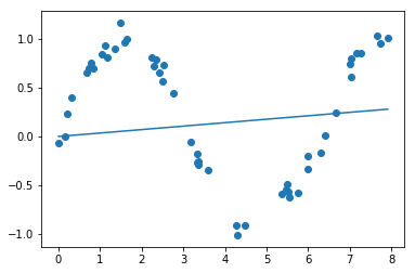
Running simple linear Regression first using statsmodel OLS

Although simple linear line won’t fit our $x$ data still let’s see how it performs.

\[y = b_0+ b_1x\]

where $b_0$ is bias and $ b_1$ is weight for simple Linear Regression equation.

Statsmodel provides OLS model (ordinary Least Sqaures) for simple linear regression.

import statsmodels.api as sm

model = sm.OLS(y, x).fit()
ypred = model.predict(x) 

plt.scatter(x,y)
plt.plot(x,ypred)

Generate Polynomials

Clearly it did not fit because input is roughly a sin wave with noise, so at least 3rd degree polynomials are required.

Polynomial Regression for 3 degrees:

\[y = b_0 + b_1x + b_2x^2 + b_3x^3\]

where $b_n$ are biases for $x$ polynomial.

This is still a linear modelâ€”the linearity refers to the fact that the coefficients $b_n$ never multiply or divide each other.

Although we are using statsmodel for regression, we’ll use sklearn for generating Polynomial features as it provides simple function to generate polynomials

from sklearn.preprocessing import PolynomialFeatures
polynomial_features= PolynomialFeatures(degree=3)
xp = polynomial_features.fit_transform(x)
xp.shape

(50, 4)

Running regression on polynomials using statsmodel OLS

import statsmodels.api as sm

model = sm.OLS(y, xp).fit()
ypred = model.predict(xp) 

ypred.shape

(50,)

plt.scatter(x,y)
plt.plot(x,ypred)

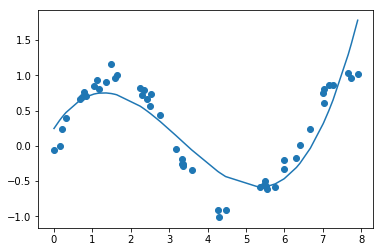
Looks like even degree 3 polynomial isn’t fitting well to our data

Let’s use 5 degree polynomial.

from sklearn.preprocessing import PolynomialFeatures
polynomial_features= PolynomialFeatures(degree=5)
xp = polynomial_features.fit_transform(x)
xp.shape

model = sm.OLS(y, xp).fit()
ypred = model.predict(xp) 

plt.scatter(x,y)
plt.plot(x,ypred)

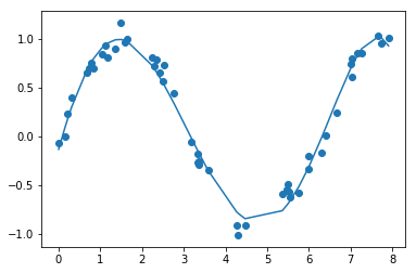
5 degree polynomial is adequatly fitting data. If we increase more degrees, model will overfit.

Model Summary

As I mentioned earlier, statsmodel provided descriptive statistics of model.

model.summary()

OLS Regression Results
Dep. Variable:	y	R-squared:	0.974
Model:	OLS	Adj. R-squared:	0.972
Method:	Least Squares	F-statistic:	336.2
Date:	Fri, 05 Apr 2019	Prob (F-statistic):	7.19e-34
Time:	11:59:50	Log-Likelihood:	44.390
No. Observations:	50	AIC:	-76.78
Df Residuals:	44	BIC:	-65.31
Df Model:	5
Covariance Type:	nonrobust

	coef	std err	t	P>\|t\|	[0.025	0.975]
const	-0.1327	0.070	-1.888	0.066	-0.274	0.009
x1	1.5490	0.184	8.436	0.000	1.179	1.919
x2	-0.4651	0.149	-3.126	0.003	-0.765	-0.165
x3	-0.0921	0.049	-1.877	0.067	-0.191	0.007
x4	0.0359	0.007	5.128	0.000	0.022	0.050
x5	-0.0025	0.000	-6.954	0.000	-0.003	-0.002

Omnibus:	1.186	Durbin-Watson:	1.315
Prob(Omnibus):	0.553	Jarque-Bera (JB):	1.027
Skew:	0.133	Prob(JB):	0.598
Kurtosis:	2.351	Cond. No.	1.61e+05

Warnings:
[1] Standard Errors assume that the covariance matrix of the errors is correctly specified.
[2] The condition number is large, 1.61e+05. This might indicate that there are
strong multicollinearity or other numerical problems.

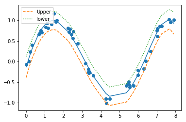
Plotting lower and upper confidance intervals

wls_prediction_std calculates standard deviation and confidence interval for prediction.

from statsmodels.sandbox.regression.predstd import wls_prediction_std
_, upper,lower = wls_prediction_std(model)

plt.scatter(x,y)
plt.plot(x,ypred)
plt.plot(x,upper,'--',label="Upper") # confid. intrvl
plt.plot(x,lower,':',label="lower")
plt.legend(loc='upper left')

Source

You can find above Jupyter notebook here

Prasad Ostwal